
05 - Reciprocal BLAST Hits (RBH)
Introduction
This notebook presents an example of programmatic use of BLAST to solve a biological problem: which gene features in a set of organisms are likely to be orthologues.
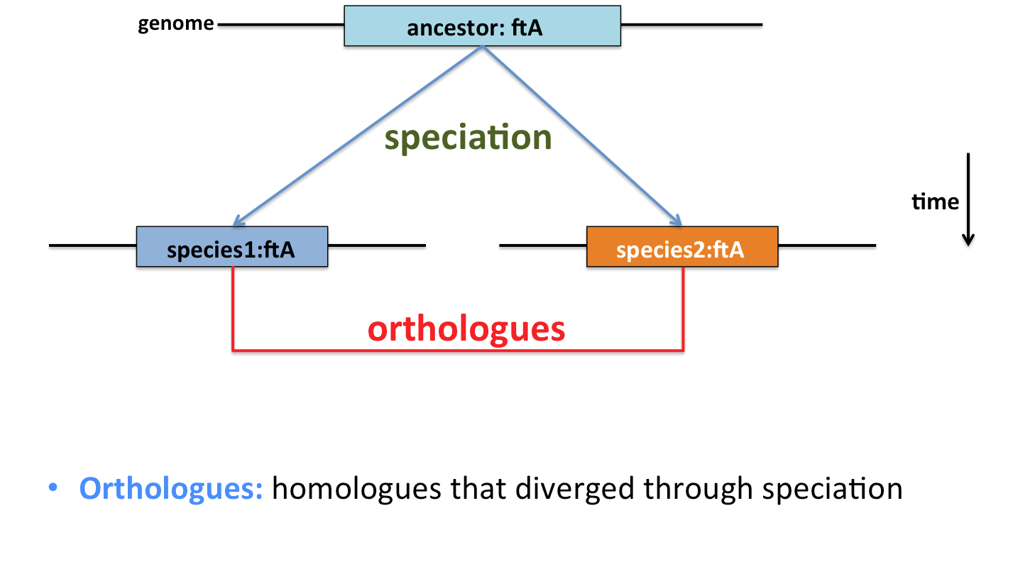
The term orthologue originally applied to features that derived from a common ancestor, and diverged through speciation. Where an unambiguous sequence counterpart can be identified in each of two diverged organisms, this may be taken to imply that the sequences are orthologues.
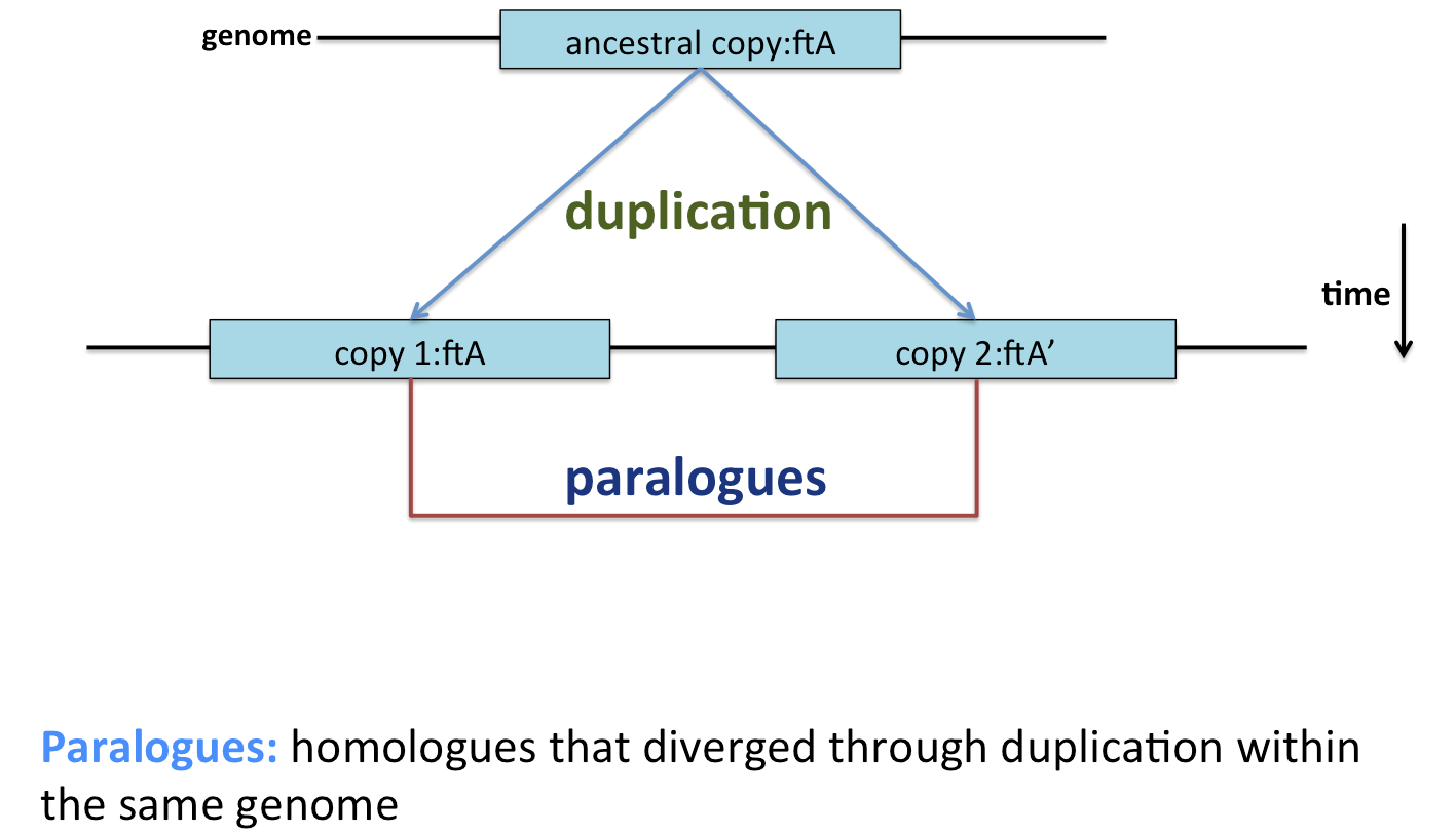
Biology is rarely that simple, however. In reality, gene duplication and gene transfer events complicate the picture. Gene duplication results in two copies of a gene being made, theoretically allowing the function of one to diverge. This may occur multiple times, and any (or no) copies may be retained. Alternatively, gene transfer from one organism to another may displace the inherited gene, or make it appear as though a gene was acquired through inheritance when it was not.
Despite these and other complication, the identification of reciprocal best hits for gene products is a good first approximation to the identification of orthologues in two or more organisms. It forms the basis for many orthology-finding tools, such as MCL, OrthoMCL and OrthoFinder. It can be carried out by carrying out BLAST+ searches using a short program, and this will be illustrated below.
Python imports
To interact with the local installation of BLAST, we will use the free Biopython programming tools. These provide an interface to interact with BLAST, run jobs, and to read in the output files.
- to collate the
BLASTsearch results as dataframes/tables for analysis, we will use thepandaspackage. - to graph the downstream results, we will use the
seabornvisualisation package.
We import these tools, and some standard library packages for working with files (os) below.
# Show plots as part of the notebook and make tools available
%matplotlib inline
import matplotlib.pyplot as plt

# Standard library packages
import os

# Import Numpy, Pandas and Seaborn
import numpy as np
import pandas as pd
import seaborn as sns

# Import Biopython tools for running local BLASTX
from Bio.Blast.Applications import NcbiblastpCommandline

# Colour scale transformation
from matplotlib.colors import LogNorm
Reciprocal Best BLAST Hits
A procedure for identifying reciprocal best hits between the protein complements of two organisms proceeds as follows:
1. Identify protein sets
- Take all the protein sequences from organism 1, and call this $S_1$
- Take all the protein sequences from organism 2, and call this $S_2$
2. Conduct forward and reverse BLAST searches
- Use
BLAST+to query the proteins from $S_1$ against those in $S_2$. These are the forward results. - Use
BLAST+to query the proteins from $S_2$ against those in $S_1$. These are the reverse results.
3. Identify forward best hits
- Consider each query sequence from $S_1$ in turn, and from the forward results identify the 'best match' in $S_2$.
- Make a table associating each sequence from $S_1$ with its best match in $S_2$. These are the forward best hits
4. Identify reverse best hits
- Consider each query sequence from $S_2$ in turn, and from the reverse results identify the 'best match' in $S_1$.
- Make a table associating each sequence from $S_2$ with its best match in $S_1$. These are the reverse best hits
5. Identify RBH
- Consider each query sequence (call this $p_1$) from $S_1$ in turn, and from the forward best hits table identify its 'best match' in $S_2$ (call this $p_2$).
- Check the reverse best hits table to find the 'best match' in the reverse direction for $p_2$.
- If this 'best match' in the reverse direction is $p_1$, then $p_1$ and $p_2$ are reciprocal best matches.
We will write code to do this analysis in the cells below.
Using local BLAST for pairwise RBH analysis
You need firstly to identify our two input protein sets: these are FASTA format multiple sequence files describing protein sets from two Kitasatospora isolates:
data/kitasatospora/GCA_001424875.1_Root107_protein.faadata/kitasatospora/GCA_001429805.1_Root187_protein.faa
and, as you did in notebook 03, construct and execute a local BLASTP search of each protein set against the other. For ease of processing, you will obtain BLAST results in tabular format.
# Define input and output directories
datadir = os.path.join('data', 'kitasatospora')
outdir = os.path.join('output', 'kitasatospora')
os.makedirs(outdir, exist_ok=True)

# Define input file paths
s1 = os.path.join(datadir, 'GCA_001424875.1_Root107_protein.faa')
s2 = os.path.join(datadir, 'GCA_001429805.1_Root187_protein.faa')

# Define output BLAST results
fwd_out = os.path.join(outdir, '05-fwd-results.tab')
rev_out = os.path.join(outdir, '05-rev-results.tab')
We can use two features of command-line BLAST that make our job easier later.
- We will restrict the number of matches to be returned to 1, by using the
-max_target_seqsargument. This will only report the best database hit to each query. We will not need to build a separate "best hit table". - We will ask only for specific information in the returned results, using the
-outfmtargument to recover: query ID, subject ID, percentage identity, percentage coverage, alignment score, and alignment E-value. (See theblastp -helpoutput for more information on these options).
# Create BLAST command-lines for forward and reverse BLAST searches
fwd_blastp = NcbiblastpCommandline(query=s1, subject=s2, out=fwd_out,
                                   outfmt="\'6 qseqid sseqid pident qcovs qlen slen length bitscore evalue\'",
                                   max_target_seqs=1)
rev_blastp = NcbiblastpCommandline(query=s2, subject=s1, out=rev_out,
                                   outfmt="\'6 qseqid sseqid pident qcovs qlen slen length bitscore evalue\'",
                                   max_target_seqs=1)

# Inspect command-lines
print("FORWARD: %s" % fwd_blastp)
print("REVERSE: %s" % rev_blastp)
# THIS CELL RUNS LARGE LOCAL BLAST SEARCHES
# IT IS SKIPPED BY DEFAULT

# Run BLAST searches
# !! Uncomment to run local BLAST searches !!
#fwd_stdout, fwd_stderr = fwd_blastp()
#rev_stdout, rev_stderr = rev_blastp()

# Check STDOUT, STDERR
#print("FWD STDOUT: %s" % fwd_stdout)
#print("FWD STDERR: %s" % fwd_stderr)
#print("REV STDOUT: %s" % rev_stdout)
#print("REV STDERR: %s" % rev_stderr)
Loading BLAST results
Once the BLAST searches are finished, you can load the tabular format results into two pandas dataframes, so that the output can be modified and inspected.
The BLAST output does not come with column headers in the file, so we have to add these ourselves, to match the columns requested in the original BLAST query.
# PRECALCULATED BLAST RESULTS
# COMMENT OUT THESE TWO LINES IF YOU WANT TO USE THE RESULTS FROM THE CELL ABOVE
fwd_out = os.path.join('prepped', 'kitasatospora', '05-fwd-results.tab')
rev_out = os.path.join('prepped', 'kitasatospora', '05-rev-results.tab')

# Load the BLAST results into Pandas dataframes
fwd_results = pd.read_csv(fwd_out, sep="\t", header=None)
rev_results = pd.read_csv(rev_out, sep="\t", header=None)

# Add headers to forward and reverse results dataframes
headers = ["query", "subject", "identity", "coverage",
           "qlength", "slength", "alength",
           "bitscore", "E-value"]
fwd_results.columns = headers
rev_results.columns = headers
Normalised bit score, and coverage
The bitscore reported by BLAST is the sum of the qualities of the aligned symbols over the whole alignment. This is an accurate measure of the alignment strength, but long sequences tend to have higher bitscores than short sequences, even when the matches are of about the same quality. To correct for this length effect, we can calculate a normalised bitscore where:
$$\textrm{normalised bitscore} = \frac{\textrm{bitscore}}{\textrm{query length}}$$
This makes comparisons of bitscore between proteins of different lengths fairer.
Calculations using pandas columns
Rather than looping over every item in a pandas dataframe column, it is possible to carry out calculations on entire columns in one action. So, to divide the contents of the bitscore column by the contents of the qlength column in the fwd_results dataframe, on a row-by-row basis, we can use the Python code:
norm_bitscore = fwd_results.bitscore/fwd_results.qlength
The query and subject sequences in a BLAST alignment may not be of the same length, so it is possible that an alignment that covers the whole of one of the sequences may only cover a small part of the other sequence (e.g. if the query sequence is a single domain protein, and that domain is part of a multi-domain protein subject sequence). That is to say, for the same alignment, the coverage of the query and the subject sequences can differ. BLAST+ only reports the query coverage, so we must calculate subject coverage ourselves.
We can define two more columns in the dataframe:
$$\textrm{query coverage} = \frac{\textrm{alignment length}}{\textrm{query length}}$$ $$\textrm{subject coverage} = \frac{\textrm{alignment length}}{\textrm{subject length}}$$
# Create a new column in both dataframes: normalised bitscore
fwd_results['norm_bitscore'] = fwd_results.bitscore/fwd_results.qlength
rev_results['norm_bitscore'] = rev_results.bitscore/rev_results.qlength

# Create query and subject coverage columns in both dataframes
fwd_results['qcov'] = fwd_results.alength/fwd_results.qlength
rev_results['qcov'] = rev_results.alength/rev_results.qlength
fwd_results['scov'] = fwd_results.alength/fwd_results.slength
rev_results['scov'] = rev_results.alength/rev_results.slength

# Clip maximum coverage values at 1.0
fwd_results['qcov'] = fwd_results['qcov'].clip_upper(1)
rev_results['qcov'] = rev_results['qcov'].clip_upper(1)
fwd_results['scov'] = fwd_results['scov'].clip_upper(1)
rev_results['scov'] = rev_results['scov'].clip_upper(1)
# Inspect the forward results data
fwd_results.head()
# Inspect the reverse results data
rev_results.head()
Visualising one-way match results
Using the seaborn package, you can summarise elements of this data visually, to get some insight into an organism-vs-organism BLAST search. For instance, a single line of code can produce a distribution plot (kernel density estimate, and histogram) of the bitscore for each BLAST hit. The bitscore encapsulates the quality of the match, and is a single measure that reflects the number of similar residues in the alignment, and their similarity.
# Set up the figure
f, axes = plt.subplots(1, 2, figsize=(14, 7), sharex=True)
sns.despine(left=True)

# Plot distribution of forward and reverse hit bitscores
sns.distplot(fwd_results.norm_bitscore, color="b", ax=axes[0], axlabel="forward normalised bitscores")
sns.distplot(rev_results.norm_bitscore, color="g", ax=axes[1], axlabel="reverse normalised bitscores");

The two plots that result from this code show the distributions of the one-way best hit BLAST bitscores.
A second plot that is useful for interpretation is the heatmap/2D density plot of query sequence coverage and subject sequence coverage:
# Plot 2D density histograms
# !! YOU DO NOT NEED TO UNDERSTAND THIS CODE TO FOLLOW THE LESSON !!

# Calculate 2D density histograms for counts of matches at several coverage levels
(Hfwd, xedgesf, yedgesf) = np.histogram2d(fwd_results.qcov, fwd_results.scov, bins=20)
(Hrev, xedgesr, yedgesr) = np.histogram2d(rev_results.qcov, rev_results.scov, bins=20)

# Create a 1x2 figure array
fig, axes = plt.subplots(1, 2, figsize=(15, 6), sharex=True, sharey=True)

# Plot histogram for forward matches
im = axes[0].imshow(Hfwd, cmap=plt.cm.Blues, norm=LogNorm(),
                    extent=[xedgesf[0], xedgesf[-1], yedgesf[0], yedgesf[-1]],
                    origin='lower', aspect=1)
axes[0].set_title("Forward")
axes[0].set_xlabel("query")
axes[0].set_ylabel("subject")

# Plot histogram for reverse matches
im = axes[1].imshow(Hrev, cmap=plt.cm.Blues, norm=LogNorm(),
                    extent=[xedgesr[0], xedgesr[-1], yedgesr[0], yedgesr[-1]],
                    origin='lower', aspect=1)
axes[1].set_title("Reverse")
axes[1].set_xlabel("query")
axes[1].set_ylabel("subject")

# Add colourbars
fig.colorbar(im, ax=axes[0])
fig.colorbar(im, ax=axes[1]);

- Most one-way matches for this data are at 100% query coverage and 100% subject coverage
- The remaining matches can be classified as either 'on the diagonal' or 'off the diagonal'
- Hits 'on the diagonal' have approximately the same coverage in query and subject sequences: these are likely diverged proteins
- Hits 'off the diagonal' have more coverage in either the query or subject sequence: these may be single-domain matches, poor alignments, or some other result that is unlikely to be a very good match.
It is unlikely that off-diagonal hits are one-to-one matches between orthologues.
Identifying reciprocal best matches
- For each query sequence named in
fwd_results.query, there is a single subject sequence named in thefwd_results.subjectcolumn (though there may be several rows, reflecting multiple alignments between the same subject and query). - The two dataframes
fwd_resultsandrev_resultsare merged such that rows are combined whenfwd_results.subjectis the same asrev_results.query. This produces a new dataframe we will callrbbh, where the forward results query and subject columns are renamedquery_xandsubject_x, while the reverse results query and subject columns are renamedquery_yandsubject_y. - Reciprocal best hits are then those where the value in
query_xmatches the value insubject_y. - All rows where
query_xdoes not matchsubject_yare not reciprocal best hits, so these are discarded. - All rows containing duplicate hits between the same query and subject sequences are grouped into a single row, taking the largest value for each column in that group.
Applying this defined procedure (an algorithm) leaves us with a single dataframe describing the reciprocal best hits for these two gene sets, in the variable rbbh.
# Merge forward and reverse results
rbbh = pd.merge(fwd_results, rev_results[['query', 'subject']],
                left_on='subject', right_on='query',
                how='outer')

# Discard rows that are not RBH
rbbh = rbbh.loc[rbbh.query_x == rbbh.subject_y]

# Group duplicate RBH rows, taking the maximum value in each column
rbbh = rbbh.groupby(['query_x', 'subject_x']).max()
# Inspect the results
rbbh.head()
Visualising RBH results
Now that we have RBH results, we can produce similar visualisations to those we used for the one-way hits, to see what has changed.
First, we produce a distribution plot of the normalised bitscores, using seaborn's distplot() function:
# Plot distribution of RBH bitscores
sns.distplot(rbbh.norm_bitscore, color="b", axlabel="RBH normalised bitscores");

What does the 2D distribution of coverage look like? We can plot this, as before:
# Plot 2D density histograms
# !! YOU DO NOT NEED TO UNDERSTAND THIS CODE TO FOLLOW THE LESSON !!

# Calculate 2D density histograms for counts of matches at several coverage levels
(H, xedges, yedges) = np.histogram2d(rbbh.qcov, rbbh.scov, bins=20)

# Create a 1x2 figure array
fig, ax = plt.subplots(1, 1, figsize=(6, 6), sharex=True, sharey=True)

# Plot histogram for RBBH
im = ax.imshow(H, cmap=plt.cm.Blues, norm=LogNorm(),
                 extent=[xedges[0], xedges[-1], yedges[0], yedges[-1]],
                 origin='lower', aspect=1)
ax.set_title("RBBH")
ax.set_xlabel("query")
ax.set_ylabel("subject")

# Add colourbar
fig.colorbar(im, ax=ax);

The difference here is even more striking. Almost all the matches along the diagonal, and off the diagonal, have disappeared. Taking reciprocal best matches has restricted the comparison between the two gene sets almost completely to proteins that are similar across almost their entire length. These are likely to be a good starting point for further analysis and transfer of functional annotation.
RBH For Multiple Gene Sets
In the cell below, we define five protein sequence files. If we want to conduct RBH analysis on these protein sequence sets, we need to perform BLAST searches using each of the five sequence sets as a query, against each of the other four sequence sets. This would be tedious to do by hand - especially for larger numbers of input files, so we can make the computer do all the hard work for us.
# Define input protein sequence files
infiles = ['GCA_000269985.1_ASM26998v1_protein.faa',
           'GCA_000696185.1_ASM69618v1_protein.faa',
           'GCA_000836635.1_ASM83663v1_protein.faa',
           'GCA_001424875.1_Root107_protein.faa',
           'GCA_001429805.1_Root187_protein.faa']

# Add the data directory to each of the input sequence files
infiles = [os.path.join(datadir, fname) for fname in infiles]
print(infiles)
Our goal is to generate forward and reverse blast results for each of the input files. We could approach this in several ways.
- A naïve approach would be to loop over this list of input files one at a time, as the query sequence set. Then, for each of these query sets, loop over the list of input files again, and create
BLAST+commands to conduct the searches we need.
While this approach would work, it has a couple of inefficiencies: we would need to avoid creating BLAST+ command lines to search a sequence set against itself. We'd also be looping twice over the same data, which can be slow for larger datasets.
# Firstly, we create a list of five elements, A to E:
my_list = ["A", "B", "C", "D", "E"]

# We can loop over these five elements and generate all pairs of
# letters, without having to loop over the whole list twice.
# Instead, we can loop over the whole list *once*, but each time
# we get a new element, we loop over the remaining list, and
# generate the forward- and reverse-pairs, as follows:
my_commands = []  # An empty list
for idx, element in enumerate(my_list):                  # OUTER LOOP
    print("CURRENT ELEMENT: %s" % element)
    # Now loop over the remaining elements in the list only.
    # This gives us the element we're dealing with, and a
    # second element as a comparator.
    # We build a command string, and put it in the list called
    # my_commands
    for comparator in my_list[idx+1:]:                   # INNER LOOP
        cmd1 = "{0} vs {1}".format(element, comparator)  # Create forward command
        cmd2 = "{1} vs {0}".format(element, comparator)  # Create reverse command
        my_commands += [cmd1, cmd2]                      # Add commands to list
        print("\t{0} vs {1}; {1} vs {0}".format(element, comparator))  # Print this cycle's commands

# We now have a list of nonredundant commands in my_commands:
print("my_commands:", sorted(my_commands))
In a similar way, it is possible to generate all BLAST+ commands to cover all the pairwise comparisons between each of the sequence files in infiles, with no repetition, or comparisons of a sequence set against itself.

Exercise 01 (20min)
Using the sequence file locations in the file infiles, can you:
- create a set of `BLASTP` commands as `NcbiblastpCommandline` objects that will conduct all pairwise reciprocal best hit calculations between those files? (HINT: you will need a different output filename for each comparison)
- print a list of those commands?
# SOLUTION - EXERCISE 01

# List to hold commands
my_commands = []

# Loop over input files and create forward and reverse commands
for idx, org1 in enumerate(infiles):
    for org2 in infiles[idx+1:]:
        fwd_out = "{0}_vs_{1}".format(os.path.split(org1)[-1],
                                      os.path.split(org2)[-1])      # Forward output file
        rev_out = "{1}_vs_{0}".format(os.path.split(org1)[-1],
                                      os.path.split(org2)[-1])      # Reverse output file
        fwd_blastp = NcbiblastpCommandline(query=org1, subject=org2, out=fwd_out,
                                   outfmt="\'6 qseqid sseqid pident qcovs qlen slen length bitscore evalue\'",
                                   max_target_seqs=1)  # Forward command
        rev_blastp = NcbiblastpCommandline(query=org2, subject=org1, out=rev_out,
                                   outfmt="\'6 qseqid sseqid pident qcovs qlen slen length bitscore evalue\'",
                                   max_target_seqs=1)  # Reverse commmand
        my_commands += [fwd_blastp, rev_blastp]

# Print out commands
print('\n\n'.join([str(cmd) for cmd in my_commands]))