EU referendum: interactive `bokeh` map

Introduction

This notebook exercise involves plotting the 2016 UK EU referendum results on an interactive map of the electoral regions in England, integrating data downloaded from the UK Data Service, and the UK Electoral Commission.

UK Data Service (Census Support): https://census.ukdataservice.ac.uk/
UK Electoral Commission: http://www.electoralcommission.org.uk/

You will use the pyshp Python library to interact with raw shapefile format data (a common GIS format), the pandas Python library to interact with voting data, and the bokeh Python library to render this data interactively, with data corresponding to the leave/remain vote indicated by colours of electoral regions.

pyshp: https://pypi.python.org/pypi/pyshp/
bokeh: http://bokeh.pydata.org/
shapefile format: https://en.wikipedia.org/wiki/Shapefile

2016 EU referendum results for England

Learning Outcomes¶

Import and process shapefile GIS data using pyshp
Import public .csv (electoral) data using pandas
Render GIS boundary data in an interactive bokeh plot
Colour geospatial data by results in an interactive bokeh plot

Exercise

The goal of this hands-on exercise is to generate an interactive plot of geographical boundary data for UK electoral regions, where those regions are coloured by the proportion of Remain votes received during the 2016 EU referendum.

Additional exercises for colouring the map with different data values are included at the end of the notebook.

The exercise is divided into three main sections:

Processing geographical boundary data
Processing vote data
Rendering the data together in an interactive bokeh plot

Each will involve the use of a different Python library, illustrating basic data-handling and integration.

1. Processing geographical boundary data

Introduction¶

Electoral and other regional boundaries for the UK are available at the UK Data Service. In particular, the https://census.edina.ac.uk/ site provides several datasets spanning all the nations of the UK, and boundaries relating to electoral, administrative and other regions. This data is provided in a number of formats, notably KML, MapInfo TAB, and ESRI Shapefile format.

To save time, the generalised, clipped shapefile data for England's electoral boundaries has already been downloaded, and should be contained in the England_lad_2011_gen_clipped subdirectory of this repository's data directory.

The shapefile format is moderately complex and may contain between 3 and 16 distinct files that describe elements of the data (see the Wikipedia page). In order to parse and work with this data, we will use the pyshp programming library.

Your goal is to convert the shapefile data into a set of x and y co-ordinates that define the boundaries of each region, so that they may be plotted using bokeh.

Python imports¶

You will need to use the pyshp library, which is imported with

import shapefile

# Import pyshp
import shapefile

Data locations¶

pyshp only needs to know the location of the .shp file, in order to process the entire dataset. For convenience, the location of this file is assigned to the variable boundaryshp.

boundaryshp = "../../data/England_lad_2011_gen_clipped/england_lad_2011_gen_clipped.shp"

# Define the location of the boundary shapefile data

Parsing shapefile data¶

The pyshp library has a Reader object that handles interactions with the geographical data. We create an object to represent our data with the statement

sf = shapefile.Reader(boundaryshp)

# Assign a shapefile.Reader object containing our data to the variable sf

Shapefile data is divided up into several components. The two components that concern us are shape and record data.

shape data contains a list of (x, y) co-ordinates that define the boundaries of each region contained in the dataset.
record data contains metadata describing each region in the dataset

In particular, the record data for our electoral boundaries comprises two strings: an Area_Code that cross-references to the electoral data we will load below; and the name of the region.

You will need to create two variables, separately holding the shape and record data.

These can be obtained using the shape() and records() methods of the sf object you created above.

shapes = sf.shapes()
records = sf.records()

# Read in the region shapes and records information

Question: What data type are the shapes and records variables?

# Answer the question in this cell

Question: How many shapes and records are there?

# Answer the question in this cell

From your answers to the questions above, you should see that the pyshp library has returned the same datatype for both shapes and records, and that there are the same numbers of shapes and records. This is not accidental.

The elements of the shapes and records variables are ordered such that each element of the two lists is paired, in order:

shapes[0] <-> records[0]
shapes[1] <-> records[1]
:
:
shapes[k] <-> records[k]

What do the `shape` and `record` elements look like?¶

You can inspect the shape and record elements to see what data they hold by looking at it directly, e.g. shapes[0] or records[0]. shapes[0] is of an non-standard type so Python returns only the memory address but we can use the .__dict__ attribute to get the content.

shapes[0]
shapes[0].__dict__
records[0]

# Inspect the shape and record elements

Shapes with several parts

Some UK regions are contiguous: they can be described by a single boundary that surrounds the entire region without a break. Other regions are not contiguous, but are divided into parts - separate subregions, each of which has a contiguous boundary. These need to be rendered as separate patches on the map.

The existence of several parts is indicated by inspecting the .parts attribute of any of the elements in shapes:

shapes[0].parts
shapes[2].parts

# Inspect the .parts attribute of some elements of the shapes list

You will have seen that all shapes elements have a list of parts, and that all these lists start with the value 0, e.g.:

print(shapes[3].parts)
[0]
print(shapes[0].parts)
[0, 243]

These values are offsets, indicating where the (x, y) co-ordinates start to describe a new contiguous region. Those shape elements whose .parts attributes are not [0] therefore comprise several disjoint regions that we ought to render as distinct objects in bokeh (otherwise the colour filling will not look correct).

Converting shape data into input for `bokeh`¶

To render the shape data we have loaded in bokeh, we need to separate each contiguous subregion's boundary data into two lists: x co-ordinates; and y co-ordinates. We also need to create two related lists, in the same order as the co-ordinate lists: one containing the region names, and one the region Area_Code accession.

The code to generate these lists is given in the cell below.

# The code below will process the shapes and records data imported
# using pyshp into four lists:
# region_xs: x-coords for each (sub)region boundary
# region_ys: y-coords for each (sub)region boundary
# region_names: names for each (sub)region boundary
# region_codes: Area_Codes for each (sub)region boundary

region_xs = []
region_ys = []
region_names = []
region_codes = []

# The enumerate() function attaches an index number to each element
# This helps us relate shapes to records
for idx, shape in enumerate(shapes):
    record = records[idx]  # index numbering is the same in both datasets
    # Names and Area_Codes will apply to all subregions
    name = record[-2]
    code = record[-1]
    # We'll pop from a list copy of shape.parts to get start/end co-ordinates
    offsets = list(shape.parts[:])
    p_start = offsets.pop(0)
    while len(offsets):
        p_end = offsets.pop(0)
        region_xs.append([point[0] for point in shape.points[p_start:p_end]])
        region_ys.append([point[1] for point in shape.points[p_start:p_end]])      
        region_names.append(name)
        region_codes.append(code)
        p_start = p_end
    region_xs.append([point[0] for point in shape.points[p_start:]])
    region_ys.append([point[1] for point in shape.points[p_start:]])
    region_names.append(name)
    region_codes.append(code)

Question: After this conversion, how many contiguously-bounded regions are there, in total?

# Answer the question in this cell

2. Importing EU referendum voting data

Introduction¶

The 2016 EU referendum voting data was made public by the UK Electoral Commission in .csv format.

2016 EU referendum data: download

To save time, this data has already been downloaded, and should be available as the file EU-referendum-result-data.csv in this repository's data directory.

This file contains a number of informative columns, including total size of electorate, number of ballots cast, and the number (and proportion) of votes for Leave, Remain (or spoiled).

Each row of the table represents a distinct area, corresponding to a single region in the geographical data we have already imported, but the two datasets do not exactly correspond. Some voting regions are not present in our geographical data, for example. The two datasets: geographical and electoral, can be joined using the Area_Code identifier.

Python imports¶

We will use the pandas Python library for importing and manipulating data. This imports data into DataFrames which behave in many ways like the dataframes in R (if that is familiar to you). It is conventional to import pandas as the alias pd, as follows:

import pandas as pd

# Import pandas
import pandas as pd

Data locations¶

All electoral data is contained in a single file, and for convenience the location is assigned to the variable votescsv below.

votescsv = "../../data/EU-referendum-result-data.csv"

# Define the location of the electoral data

Parsing electoral data¶

pandas provides a very helpful read_csv() function that returns a DataFrame object describing the data in a .csv file. The formatting of our electoral data happens to correspond well to the default expectations of this function, so can be read easily using:

df = pd.read_csv(votescsv)

You can see what the column headers are by inspecting the dataframe's attribute .columns:

df.columns

and see the number of rows and columns in the dataset with the attribute .shape

df.shape

You can use the .head() method of the dataframe to inspect the first few rows

df.head()

# Load the electoral data into the variable df, list the column headers,
# and find the size of the dataset

# Use the dataframe's head() method to inspect the first few rows

Converting electoral data into input for `bokeh`¶

We aim to convert the numerical data for the percentage of Remain ballots in each region into a list, like region_names or region_code, that associates that value with each contiguously-bounded geographical region.

To do this, we loop over every Area_Code in the region_code list and cross-reference it against the pandas DataFrame, building a list of Pct_Remain values from the imported table. This is done in the code below:

# This code compiles a list of percentage remain votes in the variable
# region_remain corresponding to the regions in the region_codes list.
# We loop over each code in the region_codes list, and pull out the
# Pct_Remain column entry for that code
region_remain = []
for code in region_codes:
    vote = df.loc[df['Area_Code'] == code, 'Pct_Remain']
    if vote.empty:
        vote = 0
    else:
        vote = vote.iloc[0]
    region_remain.append(vote)

# Create a list of Remain votes in the list variable region_remain

Question: Confirm that the expected number of Remain percentages are returned, and inspect the list to see what that percentage looks like for the first ten elements.

# Answer the question in this cell

3. Render an interactive bokeh plot

Introduction¶

Finally, we bring all the data together in an interactive plot that can be inspected in a web browser.

bokeh is a Python library for interactive visualisation that can be used to quickly create interactive plots. It renders in the style of D3.js.

We will integrate our geographical and electoral data into a ColumnDataSource object that can be used to generate a bokeh plot, and render this in the browser with useful visualisation options (zoom, pan, etc.) and annotation that renders with a mouseover event.

Python imports¶

By convention, and for clarity, the separate elements of bokeh are typically imported separately. Here, we will require the following elements from bokeh.plotting:

figure: the base rendering object
ColumnDataSource: an object for organising data to render in bokeh
show: a function to render the bokeh plot in a browser

using

from bokeh.plotting import figure, show, ColumnDataSource

We will want to use a mouseover information box, to tell the user what region they are looking at, and what proportion of the vote in that region was for Remain. For this we need the HoverTool model:

from bokeh.models import HoverTool

For our colour palette, we will use the RdYlBu10 Brewer palette, in the bokeh.palettes module:

from bokeh.palettes import RdYlBu10

Finally, because we are using a notebook, it is convenient to render directly in the notebook, rather than having to open a new window. We can do this with the output_notebook() function of bokeh:

from bokeh.io import output_notebook
output_notebook()

# Import plotting tools from bokeh
from bokeh.plotting import figure, show, ColumnDataSource

# Import HoverTool model from bokeh
from bokeh.models import HoverTool

# Import palette from bokeh
from bokeh.palettes import RdYlBu10

# Use the notebook for rendering, rather than opening a new tab
from bokeh.io import output_notebook

Creating colour information¶

To render colour information in our bokeh plot, we must provide colours in a list - one per bounded element, as with the region_names and region_codes data.

The Remain votes are defined as percentages in the range [0,100], with minimum and maximum somewhere on that range, so we could prefer a continuous or interpolated colour scale (rather than a palette of finite colours). Initially, however, we will plot using the RdYlBu10 Brewer palette, which will allow us to divide the Remain vote visually into 10% cohorts, which is a meaningful division.

As the proportion of Remain votes has a meaningful threshold value (50% representing a majority), we might prefer a colour scheme that changes visually in some significant way at that point. The RdYlBu10 palette has this property, with blue values indicating a Remain vote below 50%, and red values indicating a Remain vote above 50%.

bokeh palettes: examples

You can inspect palettes by printing them:

print(RdYlBu10)

# Inspect the RdYlBu10 palette

As can be seen, this palette is no more than a list of ten (well-chosen) colours in hexadecimal RGB format (as for web colours). It is possible to provide any valid list of colours to define a colour palette, and this is left as an exercise, later.

We wish to convert our electoral data into these ten colour bands, to create a list of colours - one per region - to reflect the percentage remain vote. We are effectively mapping all Remain percentages between 0% and 10% to the index 0, those between 10% and 20% to the index 1, and so on. These indices can then be used to pull out the relevant colour from the list in RdYlBu10, in the code below.

region_colors = [RdYlBu10[int(vote/10)] for vote in region_remain]

# Create a list of colours for each region, reflecting the percentage remain vote

# Inspect the first few elements of region_colors

Create `bokeh` data source¶

We create a new ColumnDataSource object, which will be placed in the variable source, and that will contain all relevant data, indexed with a name. The bokeh plot we create will be defined by reference to the names of these datasets:

x - region_xs: the x co-ordinates of each point on a (sub)region boundary
y - region_ys: the y co-ordinates of each point on a (sub)region boundary
name - region_names: the name for each (sub)region
code - region_codes: the Area_Code for each (sub)region
color - region_colors: the fill colour for each (sub)region, reflecting the vote data
remain - region_remain: the percentage remain vote for each (sub)region

We do this with the following code:

source = ColumnDataSource(data={'x': region_xs, 'y': region_ys,
                                'name': region_names, 'code': region_codes,
                                'color': region_colors, 'remain': region_remain})

# Create the ColumnDataSource and assign it to the variable source

Rendering the `bokeh` plot¶

Firstly, we define a set of JavaScript tools that will be displayed for navigation and manipulation of the interactive plot. This is provided as a comma-separated string of (restricted) tool names, and placed in the variable TOOLS:

TOOLS = "pan,wheel_zoom,box_zoom,reset,hover,save"

Next we create a figure element, with a plot title, and the tools defined in TOOLS. The figure is essentially an empty container at this point, waiting for us to tell it what to plot. We assign this to the variable p, so that we can add data/visual elements into this specific figure, to render our plot.

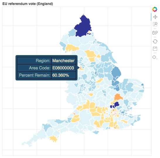
p = figure(title="EU referendum vote (England)", tools=TOOLS,
          x_axis_location=None,
          y_axis_location=None)

Now we use the patches() method of the figure p, to add our geographical regions. "Patches" are closed areas, defined by points on their boundary - for us, the x and y co-ordinates of our boundaries are contained in the x and y elements of the ColumnDataSource in the variable source. The colours of the patches/regions are contained in the color element of source.

We also add a white line boundary around our patches, so we can see the edges of regions more easily:

p.patches('x', 'y', source=source, fill_color='color',
          line_color='white', line_width=0.5)

# Create the interactive bokeh plot

QUESTION: What does the variable p now contain?

# Answer the question in this cell

You will notice that, although you have created the plot in the variable p, you still cannot see the interactive figure.

To render the interactive figure, you need to use the show() function of bokeh:

show(p)

# Render the interactive bokeh plot

The statement above renders the interactive plot in a new tab of your browser, where you can inspect the plot, seeing the regions that voted strongly to Remain as red/yellow patches, and those that voted to Leave as varying shades of blue.

Moving your mouse over the interactive plot will reveal tooltips, but these do not yet show useful data about the region or the voting information.

To add tooltip information to the interactive plot, we will use the .select_one() method of the figure p. We will create a variable called hover that implements a HoverTool presenting useful information, and which follows the mouse, reporting on the region that is directly under the mouse pointer.

hover = p.select_one(HoverTool)
hover.point_policy = "follow_mouse"

We will define which data is visible in the mouseover information box by putting (<name>, <data>) tuples in the hover.tooltips attribute - associating text labels (<name>) with columns of <data> in the ColumnDataSource we created (source).

This is done with the code below:

hover.tooltips = [("Region", "@region"),
                  ("Area Code", "@code"),
                  ("Percent Remain", "@remain%"),
                  ]

The @ syntax indicates to the tooltip that it should take values from the column in source with the name that follows the @ symbol.

You will need to use show(p); to render the interactive plot.

# Add a tooltip to the interactive plot, and render it again

EU referendum: interactive bokeh map

Introduction

Learning Outcomes¶

Exercise

1. Processing geographical boundary data

Introduction¶

Python imports¶

Data locations¶

Parsing shapefile data¶

What do the shape and record elements look like?¶

Shapes with several parts

Converting shape data into input for bokeh¶

2. Importing EU referendum voting data

Introduction¶

Python imports¶

Data locations¶

Parsing electoral data¶

Converting electoral data into input for bokeh¶

3. Render an interactive bokeh plot

Introduction¶

Python imports¶

Creating colour information¶

Create bokeh data source¶

Rendering the bokeh plot¶

Adding tooltip information¶

EU referendum: interactive `bokeh` map

What do the `shape` and `record` elements look like?¶

Converting shape data into input for `bokeh`¶

Converting electoral data into input for `bokeh`¶

Create `bokeh` data source¶

Rendering the `bokeh` plot¶